
The Basics of Back Propagation
One of the most important components of an artificial neural network are weights. These weights are what form the output based on the input.
\[a^k_i = \sum_{j=1}^{n_{k-1}} (w^k_{ij} * o^{k-1}_i) + b^k_i \qquad...(1)\] \[o^k_i = g_h(a^k_i) \qquad \qquad\qquad...(2)\] \[o^k_i = g_o(a^k_i)\qquad \qquad\qquad...(3)\]These equations pretty much describe the entire math behind the working of an ANN, also known as a multilevel perceptron. The weights are randomly assigned, based on a probability distribution like normal distribution or a gaussian distribution. Very rarely, a uniform distribution is used, but is more common for the initialization of biases.
The purpose of the weights is to allow us to get the output as close to the required output as possible — minimize the error as much as possible. To do this, we use gradient descent, a simple but effective algorithm.
Gradient Descent
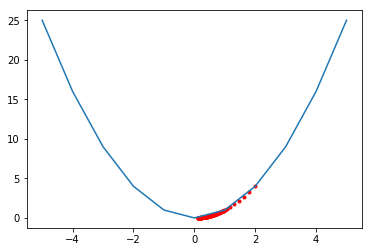
Gradient Descent is an optimization algorithm which allows one to find the minimum of an algorithm, using the gradient, often represented by $\Delta$(delta). Consider the function $f(x) = x^2$. The gradient for this one variable function is equal to its derivative, which is $2x$. The initial value of x is randomly chosen and a learning rate $\alpha = 0.01$ is used. With each iteration, x is decreased by $\alpha * \Delta (x^2)$.
The same logic is used while updating the weights. In this case the weights are updated by calculating the partial derivative of the cost with respect to the specific weight we are concerned about.
\[\frac{\partial E}{\partial w_{ij}^k} = \frac{\partial E}{\partial a_j^k}.\frac{\partial a_j^k}{\partial w_{ij}^k}\]The first part of the above formula, $\frac{\partial E}{\partial a_j^k}$ can be represented by $\delta^k_j$. The second part is easily calculated from equation (1) written above: \(\frac{\partial a_j^k}{\partial w_{ij}^k} = o_i^{k-1}\)
Hence, we have: \(\frac{\partial E}{\partial w_{ij}^k} = \delta^k_j.o_i^{k-1}\)
Calculating $\delta$ for output layer
When it comes to the last layer, we have only 1 node. Hence, we replace j with 1 in the equation given below. We use mean-squared error for E, which is one of the most common forms of error used. \(E = \frac{1}{2}\left( \hat{y} - y\right)^{2} = \frac{1}{2}\big(g_o(a_1^m) - y\big)^{2}\)
Hence, $\delta^k_j$ becomes $\delta_1^{last}$, which is \(\delta_1^{last} = \left(g_0(a_1^m) - y\right)g_o^{\prime}(a_1^m) = \left(\hat{y}-y\right)g_o^{\prime}(a_1^m)\) The partial derivative of the cost function with respect to $w_{ij}^k$ where j = 1 and k=last is \(\frac{\partial E}{\partial w_{i1}^{last}}= \delta_1^{last} o_i^{last-1} = \left(\hat{y}-y\right)g_o^{\prime}(a_1^{last})\ o_i^{last-1}\)
Calculating $\delta$ for hidden layers
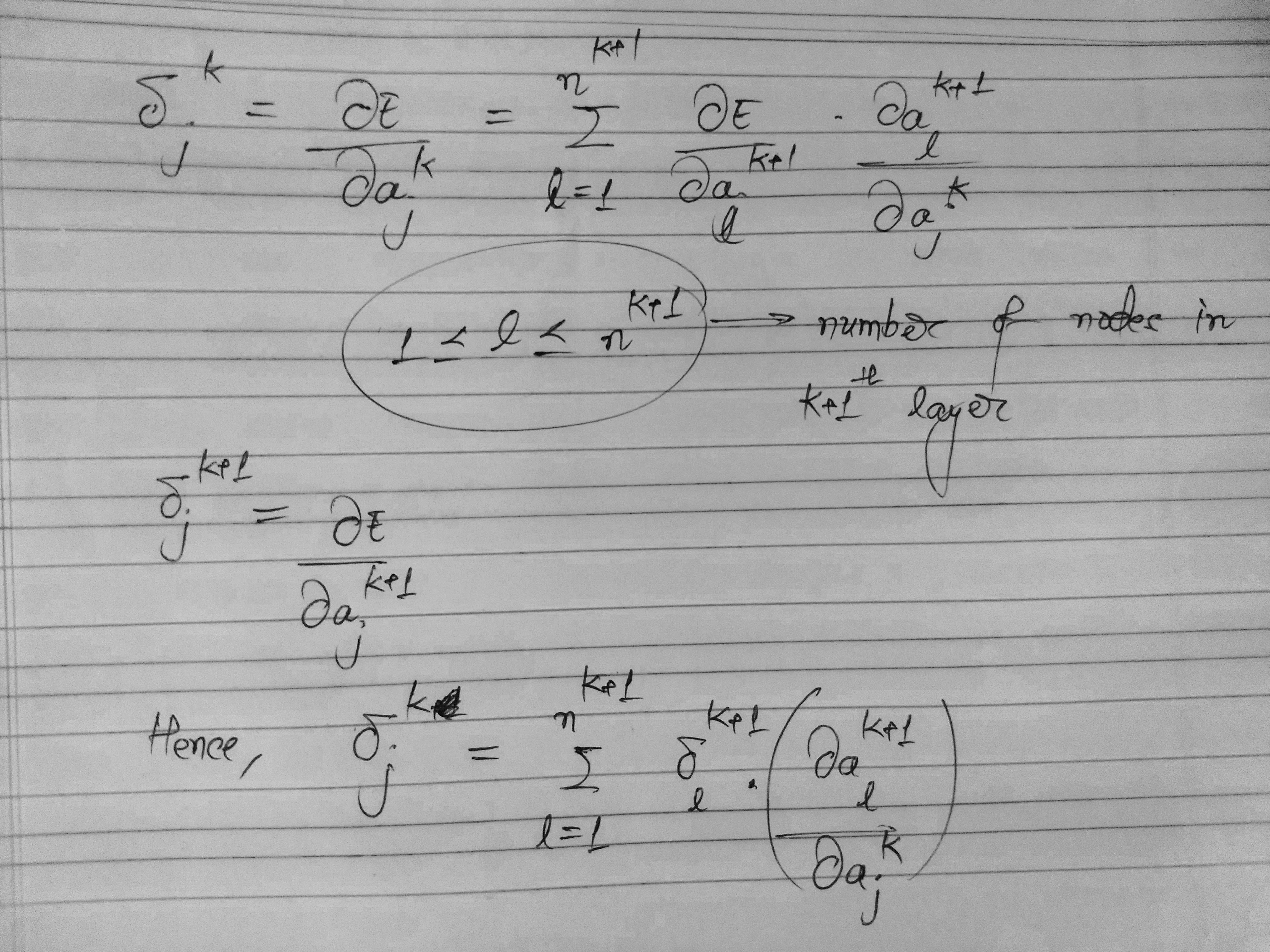 Thus, we are able to express the error of the kth layer in terms of the (k+1)th layer. Moving on to the second term $\frac{\partial a_l^{k+1}}{\partial a_{j}^{k}}$, we have the following:
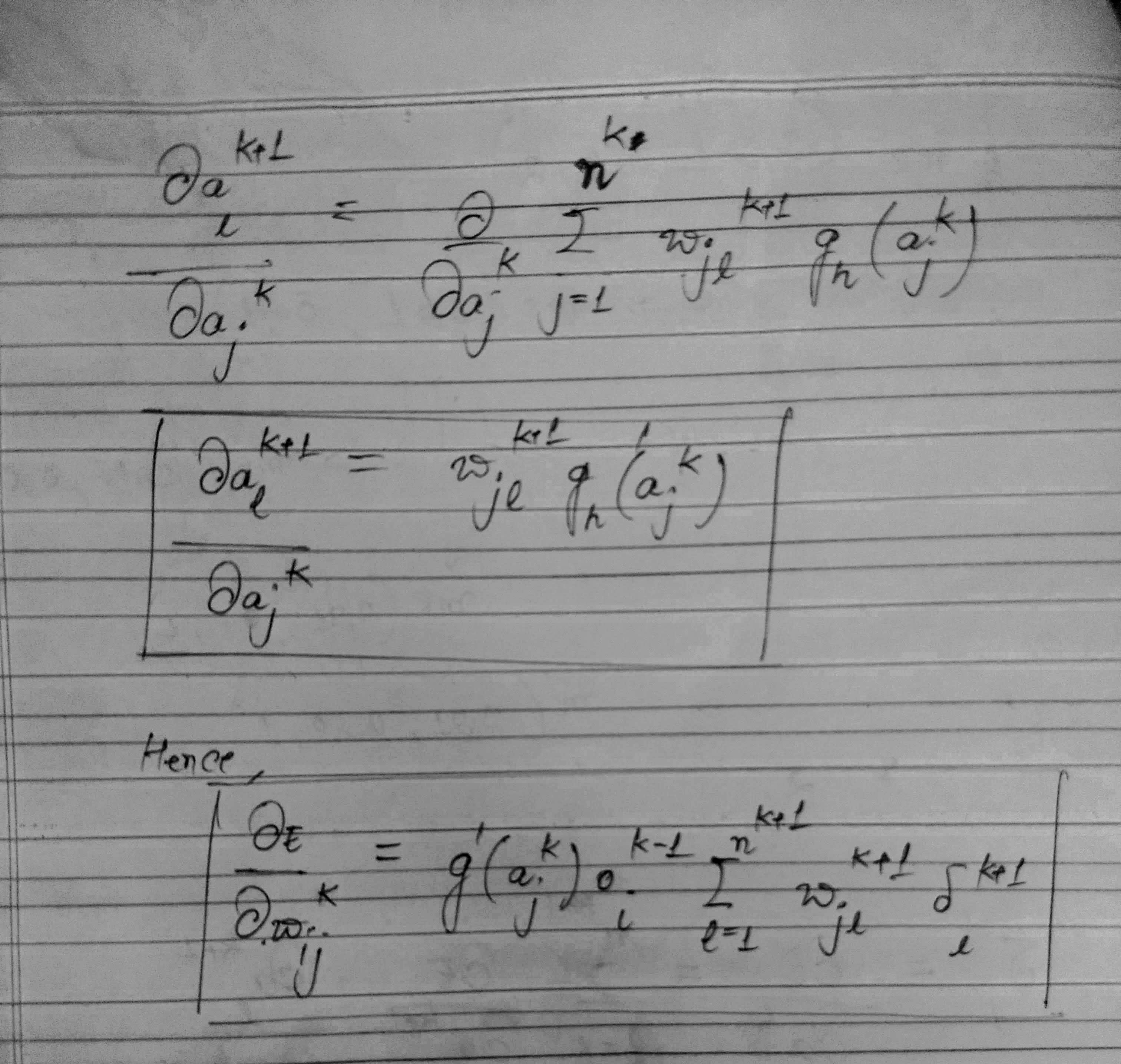
Thus, we have calculated the gradient of the cost function with respect to every weight. The weights can now be updated by decreasing them by the learning rate times the gradient.
Hence, \(\Delta w_{ij}^k = - \alpha \frac{\partial E(X, \theta)}{\partial w_{ij}^k}\)