Visualizing the Defective Chessboard problem
The defective chessboard problem is an interesting problem that is can be solved with a “divide and conquer” approach. The naive algorithm has a time complexity of $O(n^2)$.
The problem
Given a $n$ by $n$ board where $n$ is of form $2^k$ where k >= 1 (Basically n is a power of $2$ with minimum value as 2). The board has one missing cell (of size $1 \times 1$). Fill the board using trionimos tiles. A trionimo is an L-shaped tile is a $2 \times 2$ square with one cell of size 1×1 missing.
Solving the problem efficiently isn’t the goal of this post. Visualizing the board as the algorithm runs is much more interesting in my opinion, though. Lets discuss the algorithm first.
The Algorithm
As mentioned earlier, a divide-and-conquer (DAC) technique is used to solve the problem. DAC entails splitting a larger problem into sub-problems, ensuring that each sub-problem is an exact copy of the larger one, albeit smaller. You may see where we are going with this, but lets do it explicitly.
The question we must ask before writing the algorithm is: is this even possible? Well, yes. The total number of squares on our board is $n^2$, or $4^k$. Removing the defect, we would have $4^k - 1$, which is always a multiple of three. This can be proved with mathematical induction pretty easily, so I won’t be discussing it.
The base case
Every recursive algorithm must have a base case, to ensure that it terminates. For us, lets consider the case when $n$, $2^k$ is 2. We thus have a $2 \times 2$ block with a single defect. Solving this is trivial: the remaining 3 squares naturally form a trionimo.
The recursive step
To make every sub-problem a smaller version of our original problem, all we have to do is add our own defects, but in a very specific way. If you take a closer look, adding a “defect” trionimo at the center, with one square in each of the four quadrants of our board, except for the one with our original defect would allow use to make four proper sub-problems, at the same time ensuring that we can solve the complete problem by adding a last trionimo to cover up the three pseudo-defective squares we added.
Once we are done adding the “defects”, recursively solving each of the four sub-problems takes us to our last step, which was already discussed in the previous paragraph.
The combine step
After solving each of the four sub-problems and putting them together to form a complete board, we have 4 defects in our board: the original one will lie in one of the quadrants, while the other three were those we had intentionally added to solved the problem using DAC. All we have to do is add a final trionimo to cover up those three ‘defects’ and we are done.
Thus, the recursive equation for time complexity becomes:
\[\qquad T(n) = 4T(n/2) + c\]The Code
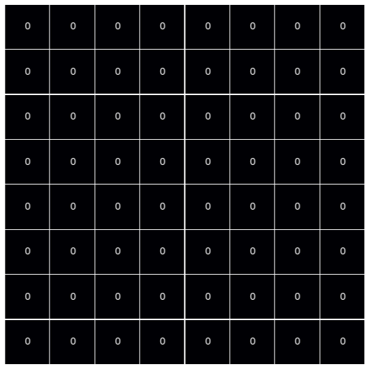
Initially, each square is represented by a 0. A ‘-1’ represents a defective square, and would appear black in the plots. Each trionimo would be displayed with a unique number, which would be incremented as more trionimos are added.
Again, the goal of the code is not optimization – its to do as much from scratch (in plain python) as possible.
I have commented the code below, so it should be pretty straight-forward.
- Importing required libraries
from random import randint
import matplotlib.pyplot as plt
import seaborn as sns
import numpy as np
The
randomlibrary is used to randomly pick a square to be defective, just for starting the problem. - Creating the board
def createboard(k): ''' k: represents the size of the board. Number of squares on the board = 2^k * 2^k ''' rows = [[] for i in range(2**k)] for i in range(2**k): rows[i] = [0] * 2**k return rows - Adding a defect randomly
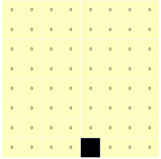
def add_defect(board): len_ = len(board) row = randint(0, len_ - 1) col = randint(0, len_ - 1) board[row][col] = -1 - Locating the defect when solving each sub-problem
def locate_defect(board, r1, c1, r2, c2): ''' (r1, c1): row, column number of upper left square of board (r2, c2): row, column number of lower right square ''' # find defective elem r = 0 c = 0 loc_ = [] for i in range(r1, r2 + 1): loc_[:] = board[i][c1:c2 + 1] if -1 in loc_: c = loc_.index(-1) + c1 r = i break # top if r <= r1 + (r2 - r1) // 2: # left if c <= c1 + (c2 - c1) // 2: return 0, r, c # right else: return 1, r, c # bottom else: # left if c <= c1 + (c2 - c1) // 2: return 2, r, c # right else: return 3, r, c - Adding trionimos
def add_trionimo(board, defect, r1, c1, r2, c2): ''' defect: integer between 0-3 representing which quadrant of the board the defect lies in. 0: top-left 1: top-right 2: bottom-left 3: bottom-right ''' global num_tri dict_ = { 0: (r1, c1), 1: (r1, c2), 2: (r2, c1), 3: (r2, c2), } num_tri += 1 for i in range(r1, r2 + 1): board[i][c1:c2+1] = [num_tri]*(r2-r1 + 1) rd, cd = dict_[defect] board[rd][cd] = -1 - Recursive Tiling Function
def tile_rec(board, r1, c1, r2, c2): global num_tri # centre coordinates dict_ = { 0: (r1 + (r2 - r1)//2, c1 + (c2 - c1)//2), 1: (r1 + (r2 - r1)//2, c1 + (c2 - c1)//2 + 1), 2: (r1 + (r2 - r1)//2 + 1, c1 + (c2 - c1)//2), 3: (r1 + (r2 - r1)//2 + 1, c1 + (c2 - c1)//2 + 1) } # locate defect quadrant drawboard(board) defect, r, c = locate_defect(board, r1, c1, r2, c2) # if board size == 2 x 2 if (r1 == r2 - 1) and (c1 == c2 - 1): add_trionimo(board, defect, r1, c1, r2, c2) return None else: # add defect to centres redo = True for value in dict_.values(): if board[value[0]][value[1]] == 0: board[value[0]][value[1]] = -1 else: redo = False if redo: board[dict_[defect][0]][dict_[defect][1]] = 0 tile_rec(board, r1, c1, r1 + (r2-r1)//2, c1 + (c2 - c1)//2), tile_rec(board, r1, c1 + (c2 - c1)//2 + 1, r1 + (r2-r1)//2, c2), tile_rec(board, r1 + (r2-r1)//2 + 1, c1, r2, c1 + (c2 - c1)//2), tile_rec(board, r1 + (r2-r1)//2 + 1, c1 + (c2 - c1)//2 + 1, r2, c2) # add last trionimo to cover defects num_tri += 1 # assume that first defect was centre redo = True for value in dict_.values(): if board[value[0]][value[1]] == -1: board[value[0]][value[1]] = num_tri else: redo = False if redo: board[dict_[defect][0]][dict_[defect][1]] = -1 - The parent tiling function
def tile(board, k):
  '''
  k: represents the size of the board.
      Number of squares on the board = 2^k * 2^k
  '''

  tile_rec(board, 0, 0, 2**k - 1, 2**k - 1)
  drawboard(board)
  return board
Visualizing
I made use of a simple seaborn heatmap to display the board. The drawboard() method creates the heatmap.
def drawboard(board, size=(8, 8), annot=True):
    '''
    size: size of plot
    annot: if true, displays the number of the trionimo a particular
        square belongs to.
    '''

    plt.figure(figsize=size)
    sns.heatmap(board, linewidths=.1, linecolor='white',
                annot=False, cmap='magma', yticklabels=False,
                xticklabels=False, cbar=False, square=True);

    sns.heatmap(board, linewidths=.1, linecolor='white',
                annot=annot, cmap='magma', yticklabels=False,
                xticklabels=False, cbar=False, square=True,
                mask=np.array(board)<0);
    plt.show()
The two heatmap calls are to more easily distinguish between defective and non-defective squares: the second heatmap has a mask which hides the defective squares, but annotates the rest, allowing us to distinguish each trionimo by number.
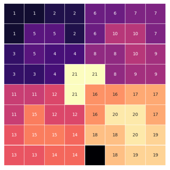
The result
I’ve dragged the post long enough. I made a gif of the output plots.